|
|
|
|

 The “canonical” understanding of complementarity is expressed
in Messiah [100, p. 154]
The description of properties of microscopic objects
in classical terms requires pairs of complementary variables; the accuracy
in one member of the pair cannot be improved without a corresponding loss
in the accuracy of the other member.  ...  It is impossible to perform measurements of position  and momentum and momentum  with uncertainties (defined by the root-mean square
deviations) with uncertainties (defined by the root-mean square
deviations)  and and  such that the product of such that the product of  is smaller than a constant unit
of action is smaller than a constant unit
of action  . .  |

the world is richer than it is possible to express
in any single language.  |

 at the beginning of the
experiment". This is often referred to as a state identification experiment.
 of states, an input alphabet
  , and a transition function
  . Instead of final states we will consider an output function
 . At each time the automaton
is in a given state
  and
is continuously emitting the output
  . The automaton remains in state
  until it receives an input signal
 , when it assumes the state
  and starts emitting
  . As we will discuss only the
simplest case when the alphabet
  , an automaton will be just a triple
  .
. 
 can be extended
to a function
  as follows:
 and
and  for all
  .
. 
 with input sequence
  is described by
  , where
  is the
function
  defined by the
following equations:


 ; recall that
  is the output function.
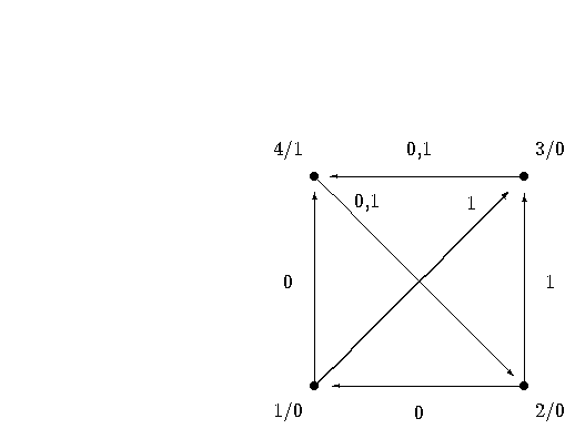
 the transition is given by the
following tables:
 ,
,  . A graphical display appears in Figure 3.5.

 with input
sequence
  leads to the output
  Indeed,


  |
  |
  |
  |
  |
  |
  |
  |

 , and following Moore [104] say
that a state
  is “indistinguishable"
from a state
  (with respect
to
  ) if every experiment performed on
  starting in state
  produces the same outcome as it would starting
in state
  . Formally,
  for all strings
  .
. 
 and
and  is to require, following Conway [46, p. 3], that for all
  ,
, 


 _
_

 , such that


There exists an automaton  such that any pair of its distinct states are
distinguishable, but there is no experiment which can determine what state
the machine was in at the beginning of the experiment. such that any pair of its distinct states are
distinguishable, but there is no experiment which can determine what state
the machine was in at the beginning of the experiment.  |
 is considered specified
if both its velocity and its position are known. Experiments can be performed
with the aim of answering either of the following:
| 1. | What was the
position of  at the beginning of the experiment? at the beginning of the experiment?
 |
| 2. | What was the
velocity of  at the beginning of the experiment? at the beginning of the experiment?
 |

| 1. | Was the automaton
in state  at the beginning of the experiment? at the beginning of the experiment?
 |
| 2. | Was the automaton
in state  at the beginning of the experiment? at the beginning of the experiment?
 |

 If there is a particle, the observer measures its position coordinate
 . If
. If  , the observer records the outcome
  , otherwise
  A similar procedure applies
for experiment B: If there is no particle, the observer records the outcome
of B as
  If there is, the
observer measures the
  -component
  of the particle’s momentum.
If
  the observer records
the outcome
  , otherwise the
outcome


